Computerized Numeric Control (CNC) technology has revolutionized modern manufacturing, enabling highly autonomous and interconnected process chains for machine tools. The foundation of CNC programming lies in standardized G-commands, which are essential for executing axis movements and control auxiliary processes, i.e. spindle on/off command. To ensure resource efficiency and optimize manufacturing processes in advance of their production, it is beneficial to evaluate their energy demand from the NC-programs as a virtual representation of the part and its processing. By estimating the energy consumption of NC programs, opportunities for optimization, such as load peak avoidance for the production schedule, can be identified.

In this context, this contribution introduces a pioneering Machine Learning (ML) approach to assess G-codes for CNC milling processes with a primary focus on understanding the energy demand associated with basic G-commands. By utilizing Latin Hypercube Sampling (LHS) as a specified Design of Experiments method, the ML model is trained with minimum experimental effort, effectively reducing the costs associated with model setup, implementation time, and deployment. This article delves into the potential of combining CNC technology with ML to enhance energy efficiency in manufacturing processes. The proposed methodology aims to pave the way for improved resource utilization and cost-effectiveness in CNC milling operations, contributing to the advancement of smart and sustainable manufacturing systems.

Energy consumption in a CNC machine originates from the spindle operation, axis feed rate, spindle speed, and the tool path interpolated by the servo drives, as well as auxiliary systems such as tool changers or cooling pumps. Hence, after a brief literature review, we provide an experimental method and the data preparation steps to train diverse ML models to predict the energy demand of an NC-operation. Then, the model performance is evaluated in a comparative study. To validate the best-performing model of our approach, we use the G-code for more elaborated parts since the initial ML model was trained with simple base G-code lines for G00 (rapid movement), G01 (linear movement), and G02 (circular movement). The paper closes by discussing the current limitations, a conclusion, and further research issues.

The paper is structured as follows: Section 2 discusses the current literature and novel aspects of this contribution. Section 3 describes the research methodology and experimental setup. This includes the Design of Experiment using LHS and the generation of training data for the ML models. Based on that, it gives an overview of the used models, the validation results, and the quality evaluation of all ML models by the measures Mean Absolute Error (MAE), Root Mean Sqaure Error (RMSE), Mean Absolute Percentage Error (MAPE), and R². After choosing a Neural Network as the best-performing model, Section 4  tested the ML model using three more complex validation parts. Sections 5 Limitations and discussion, 6 Conclusion and further research, respectively, conclude this paper by discussing limitations and further research.

2. Literature review

In previous scientific literature, there have already been attempts to predict the energy consumption of NC-programs using ML. Using characteristics like axis velocity, axis acceleration, spindle speed, spindle torque, and other machining parameters.

Borgia et al. (2014)^[1] relied on a feed-forward Neural Network with 20 inputs, two hidden layers, and one output to predict the energy consumption of machine tools during program execution. The training data for the developed two-layer Neural Network was provided by Latin Hypercube and Sobol Sampling.

Similarly, Bhinge et al. (2017)^[2] introduced a Gaussian Process Regression framework to forecast energy consumption. Their model incorporated three numerical inputs, namely feed rate, spindle speed, and depth of cut, alongside two categorical inputs, which are cutting direction and cutting strategy. The results show Normalized Mean Absolute Error values ranging from 9.5% to 13.5% for energy estimation across various blocks within the provided NC-code.

An alternative strategy was adopted in the work of Shin et al. (2017)^[3]. In this study, the authors employed a component-based technique for energy modeling designed to facilitate online optimization and real-time control. These models have the capability to predict energy usage down to the granularity of toolpaths. They are composed of both regression and Artificial Neural Network models, enabling them to anticipate the best cutting parameters for minimizing energy consumption. By selecting a milling machine case study, the authors demonstrated the efficiency of their proposed approach.

In contrast to Machine Learning methodologies, researchers have looked into analytical frameworks to predict energy demands in numerical control machining. One of these instances is presented in Lv et al. (2016)^[4]. The authors focused on motion types like auxiliary actions, air-cutting, and material removal motions to derive estimates for power consumption associated with these actions. Through a systematic Design of Experiment, various lathes and CNC machine tools were subjected to testing. The authors were then able to differentiate between the power consumption of different machines carrying out the proposed motions.

Based on their previous work, Edem and Mativenga (2017)^[5] refined their energy consumption models for machine tools to estimate the energy required to execute a CNC toolpath analytically. These models were then used to create an algorithm for energy prediction software for G-code. Their results showed that short paths for both G01 and G02/G03 were highly energy-demanding.

Also, Shin et al. (2018)^[6] use an analytical approach to model the power consumption in their work on a turning machine. They create a fine-grained model predictable up to the level of an NC program.

An alternative method of analysis was presented in the study by He et al. (2012)^[7]. The authors initially established a correlation between numerical control codes and energy consumption components of machine tools. Following this, they computed the overall energy consumption of an NC machine by summing up the energy consumption of all machine components using the spindle, axis feed, and other elements. By validating their model to actual energy measurements of two workpieces, the authors concluded that their results have the potential to enhance energy efficiency in process planning.

Brillinger et al. (2021)^[8] concentrate on developing a precise model for predicting energy consumption and power demand in CNC machine tools. They extract the NC code after manufacturing one part to train their Random Forest and Decision Tree models, analyzing 37 features, such as the cutting length of each axis. This approach aims to optimize machining strategies for lower energy consumption by predicting the power consumption for the three axes (X, Y, Z), the spindle, and the tool change system. The research underscores the importance of understanding the energy consumption of individual machining elements and explores the potential of using machine learning algorithms to make more accurate predictions. The random forest model proves to be the most accurate for predicting power consumption across all axes except for the tool change system, as evidenced by the validation part used in the testing.

Ströbel et al. (2023)^[9] employ a time series approach coupled with hybrid machine learning models to forecast energy consumption in CNC machine tool axes. The input variables, derived from the NC code, encompass axis-specific acceleration, velocity, process forces, and material removal rate, which are utilized to train three distinct Neural Networks for the XY and Z axes and the spindle. Input data encompassing the last 0.5 and the next 0.2 s is utilized in various experiments, combining air cut and material input data and air cut and material validation data. Achieving a total deviation of −10.46% to 2.25% when training with aluminum and steel and validating on the same material, the study underscores the significance of proactive monitoring and planning in energy consumption optimization, particularly in personalized production setups. Through these experiments, the research demonstrates promising results in predicting kinematic values and process forces, highlighting the necessity for a more extensive dataset to enhance prediction accuracy and applicability.

Xu et al. (2024)^[10] utilize a five-axis ultra-precision CNC machine tool, extracting axis (de-)acceleration data from the G-code to match with recorded power consumption. Employing a 1DCNN-LSTM Attention model, inputs such as axis positions, feed rate, component type, and coolant pump status are fed into the model. The most effective model achieved an MAE of 0.93. Their study introduces an intelligent G-code-based power prediction model for ultra-precision CNC machine tools, leveraging a 1DCNN-LSTM-Attention architecture. This model aims to precisely forecast energy consumption in ultra-precision machining, offering crucial insights for energy management in advanced industries. It emphasizes the significance of monitoring energy usage in ultra-precision machining and introduces a hybrid data-driven approach combining 1DCNN’s feature extraction with LSTM and attention mechanisms to capture short and long-term trends accurately.

Vishnu et al. (2020)^[11] propose a two-step approach to energy prediction in CNC machining, utilizing a Neural Network with four hidden layers and a dropout layer to forecast the actual feed rate, followed by incorporating parameters such as the length of cut in all axes, spindle speed, depth, and width of cut to predict energy consumption. With a validation RMSE of 23.1 J, their study introduces a data-driven modeling approach to optimize energy consumption during five-axis machining. This approach integrates variations in feed rate from planned values, analyzing real-time data and process plans to predict feed rates and cutting parameters, and emphasizing the importance of accurate predictions for servo motor movements. The research provides experimental data on machining conditions and toolpath strategies, aiming to empower process planners to make informed decisions for energy-efficient five-axis machining.

Pantazis et al. (2023)^[12] focus on forecasting electrical power consumption in CNC machining, particularly end milling processes. The NC code information alongside workpiece and tool geometry parameters is utilized to construct a regression model, predicting spindle acceleration, air, and material cutting power. Key features include spindle speed, duration of spindle acceleration, feed rate, depth, and width of cut. Validation, conducted with five cutting operations, attests to the model’s effectiveness, demonstrating a total power deviation ranging from −5.3% to 3.1%.

In comparison to the published literature, the specific research gaps addressed by this contribution are:

•The automated generation of single G-code commands from the LHS method to derive model training data to comprise a Neural Network based ensemble model.

•A comparative study of possibly feasible ML models to evaluate the energy demand from G-code.

•The transparent assessment of prediction errors based on three validation parts with an error propagation taking more than 500 G-code lines into account, while the ensemble model is trained with single G-code lines.

•An integrated approach combining traditional machining processes with advanced data-driven techniques, fostering a comprehensive understanding of the system and enabling the development of sustainable machining strategies.

3. Machine learning method

Based on an experimental setup, we show our ML approach in the following based on a strategy of a minimal experimental effort to derive a training data set.

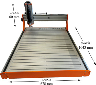
Fig. 1. CNC machine.

3.1. Experimental setup

The tests were performed using a Stepcraft M1000 CNC milling machine, which is a three-axis machine fitted with a spindle motor (see Fig. 1).

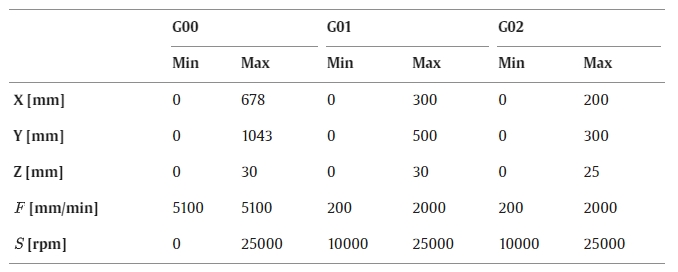
 The maximum travel distances for the axes X, Y, and Z are 678 mm, 1043 mm, and 60 mm, respectively. To ensure optimal results, the maximum feed rate of the machine should be 5100 mm/min or 85 mm/s, using the G00 command. When using commands G01 and G02, the feed should be set accordingly. Here, the feed rate ranged from 200 to 2000 mm/min, enabled by the NEMA 23 stepper motor. The spindle speed is limited to a maximum of 25000 rpm and requires a minimum of 10000 rpm to operate. The UCCNC machine control software is used for the machine’s management. The experimental search space is summarized in Table 1. 

Energy data are recorded by a Chauvin Arnoux PEL103 Power-energy logger sent by UDP to NodeRed and saved in CSV format. The data preparation and modeling are done with Python IDE.

Table 1. Machining limits defining the experimental search space.

3.2. Machine learning approach

The proposed method parses the G-code and calculates the energy consumption for each G-code line. For each G-command, the model predicts the electric power. The energy is then calculated by multiplying the total power by the time taken to machine the whole part. In particular, we follow a workflow of eight steps (see also Fig. 2):

1. Generation of Variables with LHS:

Generate X, Y, Z-coordinates, feed rate, and spindle speed using Latin hypercube sampling, ensuring a representative and efficient coverage of the design space.

2. G-code Generation:

Utilize the generated variables to create G-code sequences, incorporating motions such as G00 (rapid positioning), G01 (linear interpolation), and G02 (circular interpolation) to instruct the machining tool on its movements.

3. Energy Data Recording:

Record energy consumption data during the machining process, providing insights into the efficiency and resource utilization of the system.

4. G-code Parsing and Energy Labeling:

Parse the G-code sequences to extract relevant information and label each movement with its corresponding energy consumption, enabling a detailed analysis of the machining instructions.

5. Machine Learning Model Cross-Validation:

Perform cross-validation on various ML models to assess their performance in predicting the energy demand of the machining process based on the recorded data.

6. Training of Best-performing Algorithm:

Identify and train the most promising ML algorithm, leveraging the cross-validation results.

7. Model Evaluation on Test Data:

Evaluate the trained ML model on dedicated test data to gauge its generalization ability and ensure robust performance in real-world scenarios.

8. Validation Part Evaluation:

Assess the effectiveness of the optimized model on validation parts, validating its reliability across different instances and confirming its suitability for broader applications.

9. Permutation Feature Importance:

Identify the most important feature of the best model to assess the influence on errors.

This integrated approach combines traditional machining processes with advanced data-driven techniques, fostering a comprehensive understanding of the system and enabling the development of sustainable machining strategies.

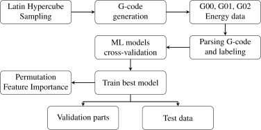
Fig. 2. Overall methodology flow chart.

3.3. Minimal data initialization method

To minimize the experimental effort with respect to the application of our proposed ML method to an industrial environment, we utilize LHS as a statistical method to generate samples from a multi-dimensional parameter space. LHS is a more efficient and evenly distributed manner compared to simple random sampling. It was proposed by McKay et al. (1979)^[13] and ensures the simultaneous stratification of all features. 

The basic idea of LHS is to divide each dimension of the parameter space into equal intervals and then randomly select one point within each interval for each dimension. This provides evenly distributed parameters in the search space. These parameters between 0 and 1 are multiplied with factors for the features, corresponding to the minimum and maximum values, resulting in the experiment parameters (see Fig. 3). 

The critical feature that distinguishes LHS from simple random sampling is that it ensures even coverage of the entire parameter space, reducing the risk of undersampling important regions. Hence, LHS is a beneficial method to generate training data for ML.

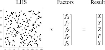
Fig. 3. LHS approach.

3.4. Training data generation and preparation

In four experiments we run 1400 G-code lines in total. The energy of the CNC machine and the spindle (separated from the CNC machine) was recorded individually. 

Fig. 4 shows the first 1000 data points of the power consumption of the CNC machine (top) and the spindle (bottom), respectively. The power measurement device recorded 10 values per second. Between each command, the movement stops for 1.5 s, which results in a drop in the energy measurements. Therefore, the energy for each G-code line can be distinguished and integrated using the trapezoidal rule (Atkinson, 1991)^[14].

To generate the features, the G-code was parsed and added to a matrix. The features used are the spindle speed and the feed rate. Additionally, the distance traveled s,  which is calculated from the G-code positions as

 

is used as a feature. With dX,dY,dZ  as the difference for each coordinate, θ  as the smaller angle between the start and end point, and r  as the radius.

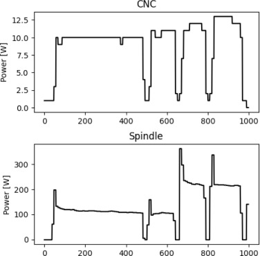
Fig. 4. Excerpt from the power measurement. Top: CNC-machine; bottom: separately monitored spindle.

All features are standardized using the StandardScaler method from the Python library scikit-learn. The data was split randomly into a training set of 80% and a test set of 20%.

3.5. Model training and evaluation

Based on the training data set, 13 different regression models are trained for each G-command (G00, G01, G02). Many approaches using Neural Networks can be found in the literature. Random Forest and Gaussian Process Regression are also used. The latter had comparatively high errors in preliminary tests, therefore this approach was not considered further. 

In addition to Random Forest, boosted decision tree algorithms (LightGBM, XGBoost, CatBoost) were used. Furthermore, multiple models from the Python library scikit-learn were included. These models are Linear Regression, Nearest Neighbor, Bayesian Ridge, Gradient Boosting, SVR, Huber, RANSAC, and TheilSen.

The metrics used to evaluate the models are Mean Absolute Error (see Eq. (2), Hodson, 2022^[15]), Root Mean Square Error (see Eq. (3), Hodson, 2022)^[16], Mean Absolute Percentage Error (see Eq. (4), Kim and Kim, 2016^[17], and R² (see Eq. (5), Kasuya, 2019^[18]), with χ_n as the predicted value, [Math Processing Error] as the target value, and [Math Processing Error] as the mean value of χ. The MAE and RMSE are commonly used metrics to evaluate the quality of models (Hodson, 2022^[19]). 

While the RMSE is mostly used for normal (Gaussian) errors, the MAE finds its optimal application in Laplacian errors. The MAPE finds common usage in practical applications because it offers a clear interpretation in terms of relative error (De Myttenaere et al., 2016^[20]). The metric R² is a measure to describe the linear relationship between two variables and is therefore called the product-moment correlation coefficient or Pearson’s correlation coefficient (

Kasuya, 2019^[21]).

The metrics MAE, RMSE, and MAPE describe the deviation between the predicted and target values, therefore the optimum value is zero. The R² however has an optimum value of one.

The used features vary within the different G-commands, with preliminary tests indicating suboptimal metrics when utilizing coordinates X, Y, and Z as features. Similarly, inferior results were observed when incorporating the differences in each coordinate (dX, dY, dZ), as well as the coordinates of G-code lines [Math Processing Error] and [Math Processing Error]. 

Optimal outcomes for G00 were achieved by employing spindle speed and traveled distance as features. For G01 and G02, the feed rate was included. It was also found in advance that adding the radius [Math Processing Error] as a feature also produces weaker results. The target of the regression model is the sum of the energy consumed by the CNC and the spindle.

To evaluate the performance of all models, the training set is used for a cross-validation consisting of 10 splits and 3 repeats. Therefore, 30 values for each model are generated. The results for G00 are shown in Fig. A.10 as boxplots. For MAE, RMSE, and MAPE, the Neural Network had the lowest mean value (MAE: 29.12, RMSE: 41.22, MAPE: 0.10, shown by a green triangle). 

Overall, the Neural Network had the highest R² score with 0.99. The metrics for G01 are shown in Fig. A.11. As with G00, the Neural Network achieved the best results, with MAE at 222.88, RMSE at 675.93, MAPE at 0.09, and R² score at 0.93. Neural Networks also achieved the best results for G02 (see Fig. A.12). The mean value of MAE is 263.67, RMSE is 626.81, MAPE is 0.08, and R² score is 0.90.

4. Results

In this Section 4, we present the results for Neural Network as the best performing model of Section 3.5. The Neural Network is trained on the data and evaluated on the test set, as mentioned in Section 3.5. The ensemble model is then utilized to predict the energy onsumption of the three validation parts.

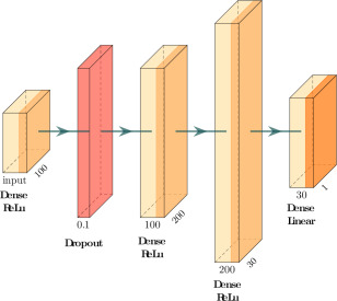
Fig. 5. Neural network architecture.

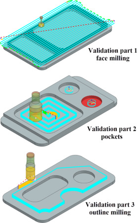
Fig. 6. Validation parts.

4.1. Ensemble model

The used Neural Network consists of 4 hidden layers (see Fig. 5). There are 2 input features for G00 and 3 inputs for G01 and G02. The inputs go into the first hidden dense layer with a ReLu activation function and 100 neurons. The output of this layer is the input for a dropout layer, which deletes 10% of the inputs. This is done to prevent overfitting (Santos and Papa, 2022^[22]). 

The third hidden layer is a dense layer with ReLu activation and 200 neurons. The last hidden layer is also a dense layer with a ReLu activation function and 30 neurons and leads into an output layer of 1 neuron with a linear activation function to predict the energy. The loss function used is the MAE with Adam as the optimizer, 300 epochs, and a batch size of 32.

The three Neural Networks for each G-command result in an ensemble model that predicts the energy demand for all G-commands of an NC-program. 

In the next step, the Neural Network is trained using the training set and evaluated on the test set. The metrics, as explained in Section 1, are listed in Table 2.  Additionally, the metrics are evaluated for the ensemble model.

Table 2. Metrics on the test data set.

4.2. Validation

To test the ensemble model of Section 4.1, three validation parts were manufactured and the energy was measured. A description of the differentiating geometrical factors of the three validation parts is detailed in Table 3.

 All parts go through three processing steps, which include face milling, pocket milling, and contour/outline milling. Generally, the geometry of the parts is similar, but the specific processing step varies from part to part. Validation part 1 has a circular outline that covers the whole profile of the workpiece. Part 2 on the other hand only has two steps on each side, whereas part 3 has a complex outline that consists of different geometries.

Pockets between all validation parts vary in form and size. Validation parts 2 and 3 have one pocket and one or more drill holes. Part one is manufactured with two different-sized pockets. Face milling for all parts is mainly the same but differs in the amount of surface area that is covered. 

All parts are shown in Fig. 6 and total around 600 G-code lines, where validation part 1 has the most lines with 664. The total number of lines is split into the different commands of G00, G01, and G02. These are assigned individually by the manufacturing software based on the operations of each part.

The absolute and relative error were chosen as evaluation metrics and can be calculated using the formula for MAE and MAPE with [Math Processing Error]. 

Table 4 lists these metrics for the three validation parts as well as the actual and predicted power consumptions. It is notable that validation parts 1 and 3 have a higher absolute and relative error compared to validation part 2.

Table 3. Milling processes for three validation parts.

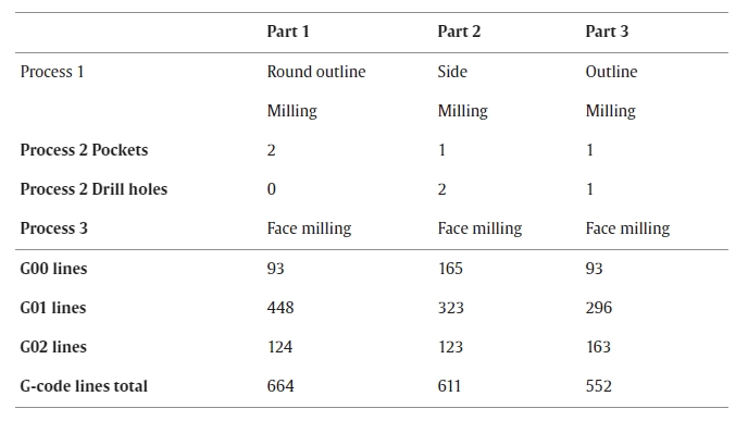
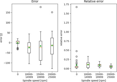
Fig. 7. Test data error and relative absolute error for G00 over different spindle speed ranges (green triangle: Mean, yellow line: Median) .

5. Limitations and discussion

The test results from Table 2 show that the MAPE for all G-commands is small (between 0.07–0.10). The MAE and RMSE for G01 and G02 are high compared to G00. This is a result of the higher mean of the total energy (G00: 435.08 J, G01: 2131.41 J, G02: 2575.55 J). One consequence of the higher errors of G01 and G02 can be a weaker energy prediction for parts with high proportions of these G-commands because of the possible accumulation of these errors.

A Permutation Feature Importance (PFI) was conducted, to analyze how relevant the input features are for the Neural Network ensemble model. The PFI is described in Breiman (2001^[23]).  The main idea is to randomly shuffle one feature of the test data set and save the results. The feature with the largest decrease in the result is the most important.

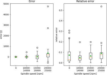
Fig. 8. Test data error and relative absolute error for G01 over different spindle speed ranges.

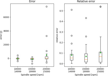
Fig. 9. Test data error and relative absolute error for G02 over different spindle speed ranges.

Table 4. Validation results.

For all three trained models, spindle speed was the most important feature. Followed by the distance for G00 and G02. For G01, the feed rate was the second most important feature.

The error ([Math Processing Error]) and the relative absolute error [Math Processing Error] in relation to the spindle speed ranges for G00 are shown in Fig. 7. 

The yellow line shows the median, the green triangle the mean value, and the black dots the outliers. In the following, the spindle speed between 10000 rpm and 14999 rpm is defined as range 1, spindle speeds from 15000 rpm to 19999 rpm are range 2, and range 3 are speeds between 20000 rpm and 25000 rpm. 

When the spindle speed is zero, the mean error is small (0.87 J), in contrast to higher spindle speeds (range 1: −22.61 J, range 2: −15.23 J, range 3: −12.42 J). The relative error remains consistently minor across all spindle speed ranges (spindle speed 0 rpm: 0.10, range 1: 0.12, range 2: 0.10, range 3: 0.06). 

However, outliers are evident in both error measures. Higher spindle speeds result in a higher range between the quantiles and an increased mean error. The relative error shows the same behavior.

Fig. 8 shows the errors for G01. Similar to G00, the average error at zero spindle speed (−5.86 J) is lower than at higher speed values ([Math Processing Error] J). Notably, the mean error within the spindle speed ranges 1 and 2 is comparatively smaller (25.45 J and 42.48 J) than the error observed in range 3 (379.44 J). Across all spindle speed ranges, the relative error is generally small (0 rpm: 0.07, range 1: 0.05, range 2: 0.07, range 3: 0.09), although a few outliers are present in each range.

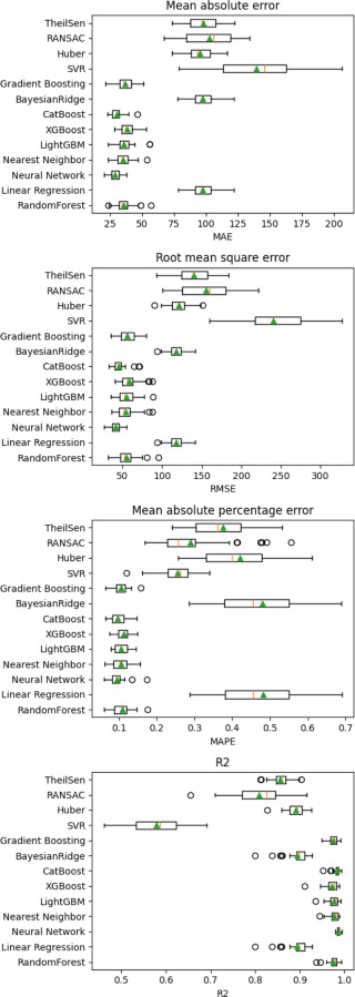
Fig. A.10. Cross-validation results G0 (green triangle: Mean, yellow line: Median) .

In Fig. 9 the errors associated with G02 are depicted. Spindle speeds lower than 20000 rpm lead to a smaller mean error (range 1: −9.44 J, range 2: −63.39 J). Spindle speeds exceeding 20000 rpm exhibit a notable mean error of 502 J, accompanied by a few outliers. However, the relative error remains consistently small across all spindle speeds, amounting to less than 0.11 (range 1: 0.08, range 2: 0.07, range 3: 0.11).

The error for range 3 is for all G-commands comparably high (−12 J to 502 J), however, the relative error is between 5% and 11%. This is a result of the higher power consumption of larger spindle speeds.

G-codes may lack the detail needed to fully address the complexities of certain machining tasks or advanced manufacturing processes. This includes factors like environmental conditions, which can significantly impact energy consumption during machining operations. 

As a result, there may be discrepancies between predicted and actual energy usage that can lead to inefficient resource allocation, increased operating costs, and greater environmental impact. Overestimation of energy demand leads to inefficient resource utilization and increased costs, while underestimation may trigger unforeseen expenses and worsen environmental degradation, especially for carbon-intensive energy sources. 

Accurate energy forecasting is critical for optimizing resource allocation, controlling costs, and reducing the environmental footprint of machining operations, underscoring the importance of precision in energy forecasting for sustainable manufacturing processes.

6. Conclusion and further research

Our contribution focuses on the derivation and validation of an ML model designed to predict the energy demand of an NC-program based on its G-code lines. 

The provided methods utilize LHS to automatically generate G-code, ensuring efficient coverage of the training data space. Based on a comprehensive data set varying the input parameter distance, spindle speed, and G-command, several ML models were trained. A Neural Network ensemble model performs best and is validated by three parts. 

The prediction loss for the entire NC-program, ranging between 552 and 664 lines of code, falls within the 0.7% to 55% range, while the overall model accuracy remains around 92% for each G-code command line.

On one side, additional research activities will focus on the optimization of the prediction model to further increase the accuracy by integrating more features. On the other side, we aim to generalize our ML approach with respect to material properties and machine-neutrality.

Funding

This work was supported by the “Bayerisches Staatsministerium für Wirtschaft, Landesentwicklung und Energie” [grant number DIK-2104-0013//DIK0248/03]. Supported by the publication fund of the Technical University of Applied Sciences Würzburg-Schweinfurt.

CRediT authorship contribution statement

Anna-Maria Schmitt: Writing – original draft, Visualization, Software, Methodology, Conceptualization. Eddi Miller: Writing – original draft, Validation, Data curation. Bastian Engelmann: Writing – review & editing, Supervision. Rafael Batres: Methodology, Investigation. Jan Schmitt: Writing – review & editing, Writing – original draft, Visualization, Funding acquisition.

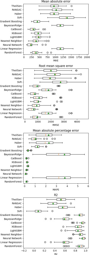
Fig. A.11. Cross-validation results G1.

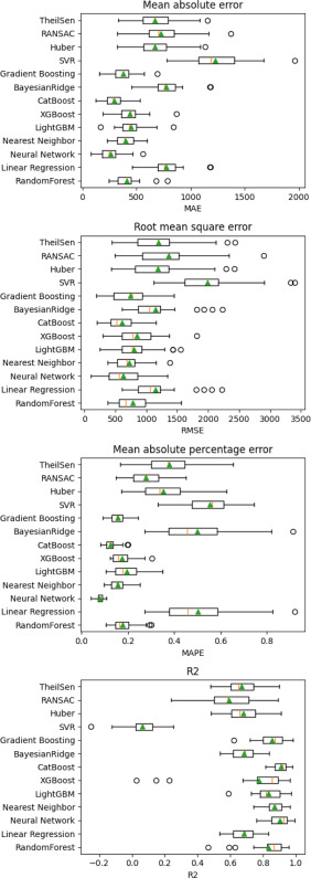
Fig. A.12. Cross-validation results G2.

Declaration of competing interest

The authors declare that they have no known competing financial interests or personal relationships that could have appeared to influence the work reported in this paper.

Appendix. Cross-validation results

Figs. A.10, A.11, and A.12 show the cross-validation results for the three G-commands.

Reference

1. [1]] Borgia S., Pellegrinelli S., Bianchi G., Leonesio M. A reduced model for energy consumption analysis in milling
2. [2] Bhinge R., Park J., Law K.H., Dornfeld D.A., Helu M., Rachuri S.Toward a generalized energy prediction model for machine tools
3. [3] Shin S.-J., Woo J., Rachuri S. Energy efficiency of milling machining: Component modeling and online optimization of cutting parameters
4. [4] Lv J., Tang R., Jia S., Liu Y. Experimental study on energy consumption of computer numerical control machine tools
5. [5] Edem I.F., Mativenga P.T. Modelling of energy demand from computer numerical control (CNC) toolpaths
6. [6] Shin S.-J., Woo J., Rachuri S., Meilanitasari P. Standard data-based predictive modeling for power consumption in turning machining
7. [7] He Y., Liu F., Wu T., Zhong F.P., Peng B. Analysis and estimation of energy consumption for numerical control machining
8. [8] Brillinger M., Wuwer M., Hadi M.A., Haas F. Energy prediction for CNC machining with machine learning
9. [9] Ströbel R., Probst Y., Deucker S., Fleischer J. Time series prediction for energy consumption of computer numerical control axes using hybrid machine learning models
10. [10] Xu Z., Selvaraj V., Min S. Intelligent G-code-based power prediction of ultra-precision cnc machine tools through 1DCNN-LSTM-attention model
11. [11] Vishnu V.S., Varghese K.G., Gurumoorthy B. Energy prediction in process planning of five-axis machining by data-driven modelling
12. [12] Pantazis D., Goodall P., Pease S.G., Conway P., West A. Predicting electrical power consumption of end milling using a virtual machining energy toolkit (V_MET)
13. [13] McKay D., Beckman R.J., Conovcr W.J. A comparison of three methods for selecting values of input variables in the analysis of output from a computer code
14. [14]  Atkinson K. An Introduction to Numerical Analysis
15. [15] Hodson T.O. Root-mean-square error (RMSE) or mean absolute error (MAE): When to use them or not
16. [16] Hodson T.O. Root-mean-square error (RMSE) or mean absolute error (MAE): When to use them or not
17. [17] Kim S., Kim H. A new metric of absolute percentage error for intermittent demand forecasts
18. [18] Kasuya E. On the Use of R and R Squared in Correlation and Regression: Technical Report
19. [19] Hodson T.O. Root-mean-square error (RMSE) or mean absolute error (MAE): When to use them or not
20. [20] De Myttenaere A., Golden B., Le Grand B., Rossi F. Mean absolute percentage error for regression models
21. [21] Kasuya E. On the Use of R and R Squared in Correlation and Regression: Technical Report
22. [22] Santos C.F.G.D., Papa J.P. Avoiding overfitting: A survey on regularization methods for convolutional neural networks
23. [23] Breiman L. Random forests